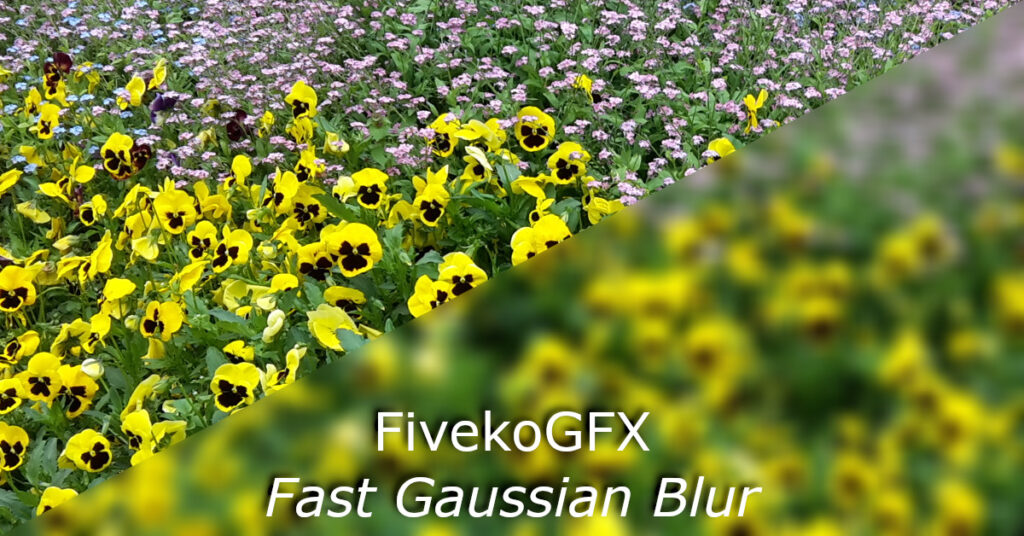
Gaussian Blur - Noise Reduction Filter

Gaussian blur is an essential part of many image processing algorithms. It serves to clear the noise in the images, as well as a general visual effect in various graphics software.

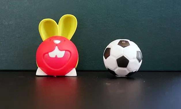
The following photo utility uses a Gaussian filter to blur images right in a web browser.

What is Gaussian blur?

Gaussian blurring is a non-uniform noise reduction low-pass filter (LP filter). The visual effect of this operator is a smooth blurry image. This filter performs better than other uniform low pass filters such as Average filter (Box blur).

How does Gaussian smoothing works?

Gaussian smooth is an essential part of many image analysis algorithms like edge detection and segmentation.

The Gaussian filter is a spatial filter that works by convolving the input image with a kernel. This process performs a weighted average of the current pixel’s neighborhoods in a way that distant pixels receive lower weight than these at the center.

The result of such low-pass filter is a blurry image with better edges than other uniform smoothing algorithms. This makes it a suitable choice for algorithms such as Canny edge detector.

Gaussian blur filter example with sigma 3 — *Left – image with some noise, Right – Gaussian blur with sigma = 3.0*

The math equations below show how to calculate the proper weights of a Gaussian kernel.

One dimensional Gaussian function

gaussian-blur-1d-shape — One-dimensional Gaussian function

Gaussian function 1D math — One-dimensional filtering kernel equation (1)

Two dimensional Gaussian function

The equation below (2) shows how to calculate two-dimensional Gaussian function:

Gaussian function 2D math — Two-dimensional filtering kernel equation (2)

Separable property

In practice, it is better to take advantage of the separable properties of the Gaussian function. This feature allows you to blur the picture in two separate steps.

This saves computing power by using a one-dimensional filtering as two separate operations. As a result, we achieve a fast blur effect by dividing its execution horizontally and vertically.

Features and applications

The list below provides a brief summary of the characteristics of the Gaussian filter:

It is a separable filter – this property can save significant computing power
Preferable choice for edge detection – using “weighted” masks makes it better than some uniform blur filters
Multiple iterations with a given filter size have the same blur effect as the larger one
Useful as a pre-processing step for image size reduction

Discrete Approximations

In many cases it is enough to use an approximation of Gaussian function. Below are examples of popular filtering masks that we often use in computer vision.

Separable Filter with Size 3×3

$\displaystyle{K}=\frac{1}{{16}}{\left[\begin{matrix}{1}&{2}&{1}\\{2}&{4}&{2}\\{1}&{2}&{1}\end{matrix}\right]}={\left[\begin{matrix}{1}&{2}&{1}\end{matrix}\right]}\frac{1}{{4}}\ast{\left[\begin{matrix}{1}\\{2}\\{1}\end{matrix}\right]}\frac{1}{{4}}$ — Discrete approximation of Gaussian filter with size 3×3

Separable Filter with Size 5×5

$\displaystyle{K}=\frac{1}{{256}}{\left[\begin{matrix}{1}&{4}&{6}&{4}&{1}\\{4}&{16}&{24}&{16}&{4}\\{6}&{24}&{36}&{24}&{6}\\{4}&{16}&{24}&{16}&{4}\\{1}&{4}&{6}&{4}&{1}\end{matrix}\right]}=\frac{1}{{16}}{\left[\begin{matrix}{1}&{4}&{6}&{4}&{1}\end{matrix}\right]}\ast\frac{1}{{16}}{\left[\begin{matrix}{1}\\{4}\\{6}\\{4}\\{1}\end{matrix}\right]}$ — Discrete approximation of Gaussian filter with kernel size 5×5

Note that when converting continuous values to discrete ones, the total sum of the kernel will be different than one. This leads to brightening or darkening of the picture, so in practice we normalize the kernel. We achieve this by dividing each of its elements by the sum of all of them.

Gaussian Filter example code

The table below provides links to sample source code in various programming languages and technologies:

Link	Description
Gaussian filter in pure JavaScript	Use native JavaScript to implement blur effect on images and pictures. No dependencies and third party libraries.
Gaussian filter in OpenGL (WebGL)	Implement image blur filter using WebGL/OpenGL technology. Simple and fast image filtering using GPU.

Image Filtering Online

You can use various image editing and analysis tools for free, here online in your browser. No registration, download and without watermarks.

References

Support Me on Ko-fi

Gaussian Blur – Noise Reduction Filter

What is Gaussian blur?